Energy price forecasting with deep learning
Introduction
Our dataset[1] is based on Spanish energy generation, weather, and price data. Energy prices in European markets are largely driven by merit order [2], which ranks power generation based on ascending order of marginal cost. Nuclear is relatively cheap but inflexible in terms of ramping output, so operates as baseload. Renewables have near-zero marginal cost at generation time and are used whenever available, while coal and gas can be turned up or down to satisfy residual demand.
The result of this structure is that renewables exert a downward pressure on prices when available, and introduce volatility, whereas times of low renewable output lead to higher and more stable prices. Spain has a slight caveat to this, with the Andasol solar plant[3] generating solar during the daytime and providing storage in molten salt, allowing energy to be exported overnight.
The objective of the deep learning model is to learn these relationships, in particular how weather forecasts for a given location translate into renewable energy availability and, in turn, influence day- ahead electricity prices.
Method
Dataset preparation
The dataset was processed in several ways. Firstly we remove features that are all zero, for example generation types that do not seem to apply to Spain, e.g. geothermal. Such columns add little to the predictive power of a model, but will needlessly increase the parameter count.
Secondly we process each feature to check for anomalies. Anomalies are detected using a rolling statistical baseline, where values deviating beyond a fixed number of standard deviations from a centred moving mean are flagged, subject to a minimum absolute deviation threshold. To avoid marking regime shifts or sustained volatility, only isolated outliers (with neighbouring points remaining in-range) are retained, with optional handling of isolated zero-valued artefacts (depending on the feature). The detection procedure is parameterised per feature (e.g. number of standard deviations) to account for the vastly different statistical profiles across variables. For weather we also incorporate known min/max records for features like pressure, to ensure there are no obviously incorrect values.
Anomalies are marked as NaN and then processed further (along with any values missing in the
original dataset). We use linear interpolation to bridge any gaps, but specify an hourly limit to this
operation (6 hours) to avoid guessing large gaps. No gaps larger than this were found.
The snow feature was re-sampled using averaging to give us hourly values. The data was so sparse for this feature that it was impractical to perform anomaly detection, so the values are used as-is.
The date and time features are cyclically encoded. The wind direction feature also required cyclical encoding, as a small shift from 360 degrees to zero would be seen by the model as a large jump, when in reality it would be a tiny direction shift.
The weather and energy datasets were then merged and split into train and test. We were careful to normalise the values on the training set only, and then apply the scalers to the test set to avoid information leakage. The scalers were then stored on disk for later use in evaluations.
The training dataset is further split into model training and model validation datasets. We ensure that the validation set contains a full calendar year of data, to ensure validation loss values contain any seasonal variances present in the data.
Model Architecture
The model comprises 3 distinct branches. Firstly, we have a CNN + LSTM combination that processes historical weather, generation and demand features. Secondly, we have a city-level atten- tion layer that attempts to weight the importance of the weather per future timestep across cities, which is then temporally encoded using a separate LSTM. Thirdly, we have a vector of historical prices (last 24 hours). Each of these branches produces learned representations which are concate- nated together, before being passed through a two-layer MLP to produce our final predictions.
Historical Demand & Weather
The inputs to the CNN are historical weather, generation and load data only, we do not include the price. The intention is that the CNN will learn local patterns and pass those to the LSTM which can then weight those local patterns against longer term patterns, whilst outputting the learned features into a fixed-size representation.
Given the short sequences we operate on within the model, it was decided that a CNN stride of 1 should be fixed so that we preserve temporal resolution and avoid implicit downsampling. The model also exposes the dropout parameter of the LSTM to allow us to tune the level of regularisation that will occur during training.
A data generation function is used to generate sequential time series for feeding into the model. There was a choice between limiting the output of this to purely data for training 23:00 predictions specifically, but the resulting training dataset was extremely small. Instead, the function strides over the dataset at a configurable rate, producing series for all times of day. The function also allows configuration of the number of trailing hours that are included in the series. See section 3 for experiments surrounding these parameters.
Future Weather
We use future weather as perfect predictions rather than pulling in historical forecasts. To exploit this, we use a combination of city-level attention and an LSTM.
The attention module allows us to model the weather spatially rather than temporally, and assign weights dynamically to each city to determine which is most important for a given hour. The attention outputs are time indexed but are spatial rather than temporal, so we use the LSTM to capture weather patterns, e.g. sustained wind, which then produces a temporal encoding of the spatially aggregated data.
This is one of the few areas of the model that could provide some level of explainability, as the output from the attention mechanism is a probability distribution which could give us insight into how the weather impacts predictions downstream.
Historical Prices
The historical prices represent the last 24 hours of price actual values, i.e. the labels from the
previous day (the labels are known after the fact, so there is no future leakage). Energy prices tend
to follow a known structure called the Duck curve[4], which was found to be present in our data,
and also explains the fairly strong performance of the “yesterday” baseline (see experiments). By
injecting historical prices into the model separately to the historical branch, we can ensure the signal
from this feature is strong, which could reduce the burden on the model of having to learn this
inherent market structure.
We hard code the historical values to 24 hours, to ensure that the model always sees a full picture of daily seasonality and aligns with the forecasting horizon.
Fusion & MLP head
Each of the branches is concatenated into a single vector before a simple two layer MLP produces our final predictions. The concatenation is the key component that allows us to inject historical prices at a later stage than the historical encoder, while the MLP is responsible for ultimately deciding how the latent variables from each branch should be represented in the final output, which is a single vector containing our 24 hourly predictions.
Experiments & Discussion
We have two broad choices to make for the model design. We could have an approach that comprises of multiple models (predicting demand and outut, feeding results to a price model) or a unified model. It was decided that a unified model was preferable. Whilst multiple models provide increased explainability in terms of what is being fed into the price model, we inherently crystallise losses when we make demand and renewable output predictions. A unified model allows for more expressivity internally for these values and may reduce the final error in the final model.
Figures 2 and 3 show the training of the specific model used for the evaluation. The curves indicate stable convergence with no evidence of overfitting. Validation loss stabilises after approximately 120 epochs, supporting the use of early stopping (see section 3.1).
The selected baselines are day ahead persistence (yesterday’s profile), seasonal naive, and a SARIMAX[5] for comparison. The SARIMAX approach factored in exogenous features provided to the model, such as weather and generation values.
The high level results are as follows.
| Name | MAE | RMSE | MAPE |
|---|---|---|---|
| Model | 3.9795 | 5.4034 | 7.31 |
| Yesterday | 5.1443 | 7.5355 | 9.81 |
| Seasonal Naive | 6.0992 | 8.9449 | 12.18 |
| SARIMAX | 13.7209 | 16.14149 | 23.13 |
The model consistently outperforms all baselines. We can see that day ahead persistence performs quite strongly, but the model reduces average error and also the severity of larger errors quite considerably. Seasonal naive is also fairly strong, but underperforms compared to yesterday. This is unsurprising, as the variance from today to yesterday in terms of weather, demand and pricing is generally more likely to be lower than comparing to the same hour last week. SARIMAX performed relatively poorly, especially given the model was provided with the same inputs as our model.
Subsequent analysis will focus on the day ahead persistence baseline given its strength compared to the other baselines. It’s also most appropriate given our model explicitly learns from yesterday’s pricing, so logically we’re seeing the effects of the model applying the exogenous variables to the problem.
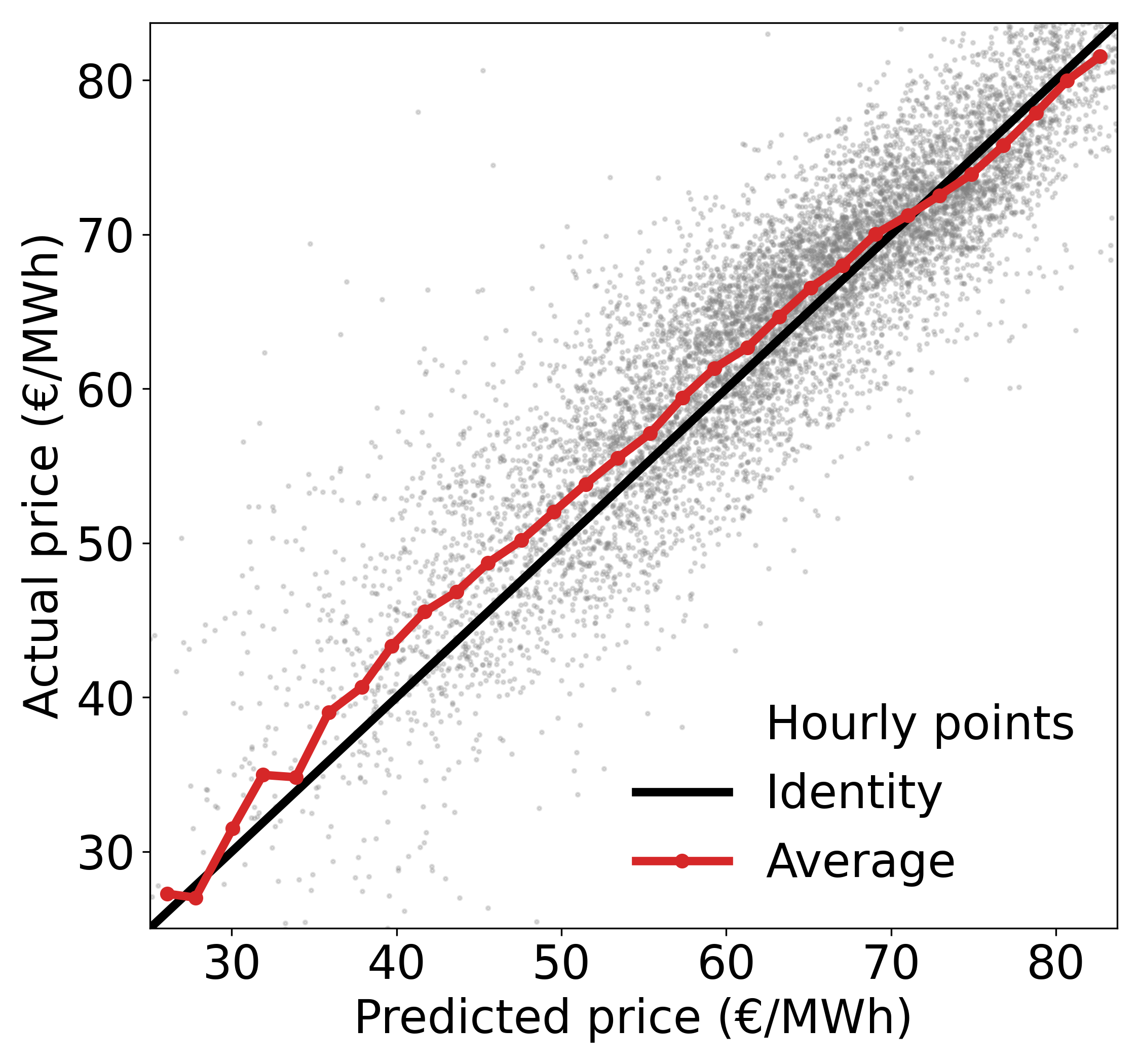
The representative month was chosen by taking the month closest to the median MAE. In this case November 2018. We can see the model performs well throughout the month, capturing the daily shape well. Inaccuracies tend to be overpredictions rather than underpredictions. This is supported by the calibration plot (figure 9) which shows good performance, but that the model was slightly skewed to overpredictions.
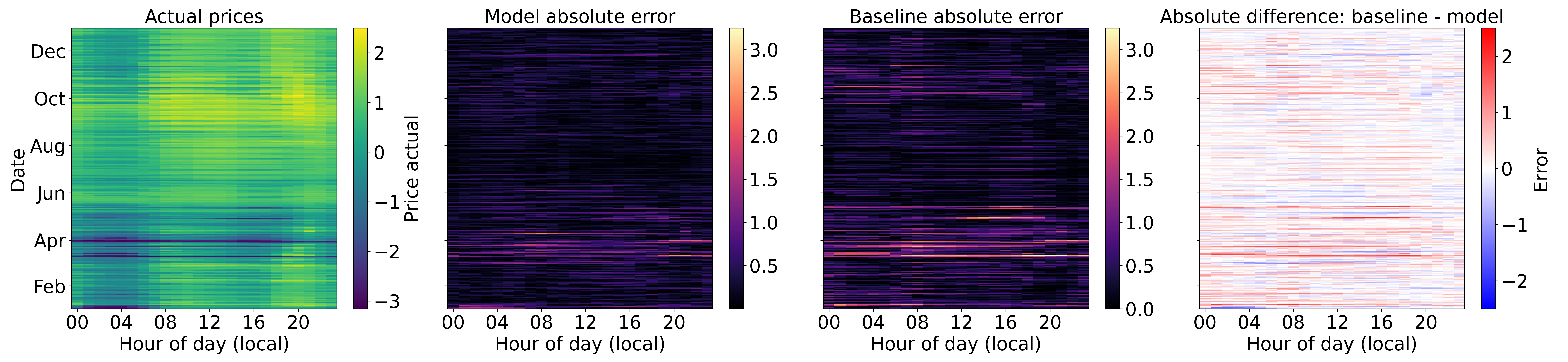
Figure 5 shows performance across the entire test set. The charts show raw price, model performance, baseline performance, and difference between model and baseline respectively. In the raw prices we can see a period of relative volatility in March in which the model performs noticeably better than the baseline. In the summer months both the model and baseline perform similarly, suggesting that prices were fairly stable in those months, likely driven by abundant stable solar energy. There’s an uptick in volatility towards the end of the year, which again is handled well by the model compared to the baseline. This view strongly suggests the model was able to use the more volatile generation types (e.g. wind) effectively to predict price.
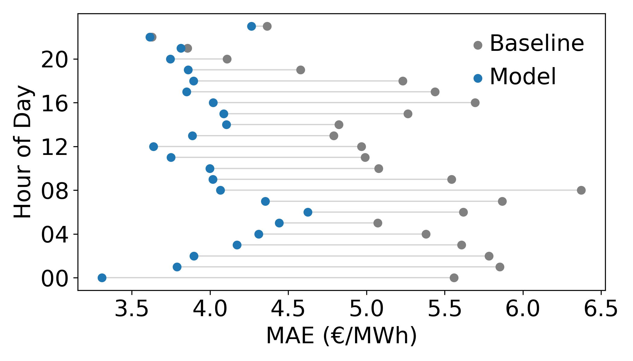
Figures 6-8 give a more detailed breakdown of performance. Figure 6 shows the hourly error of the model and the baseline. We can see the model consistently outperforms the baseline across all hours.
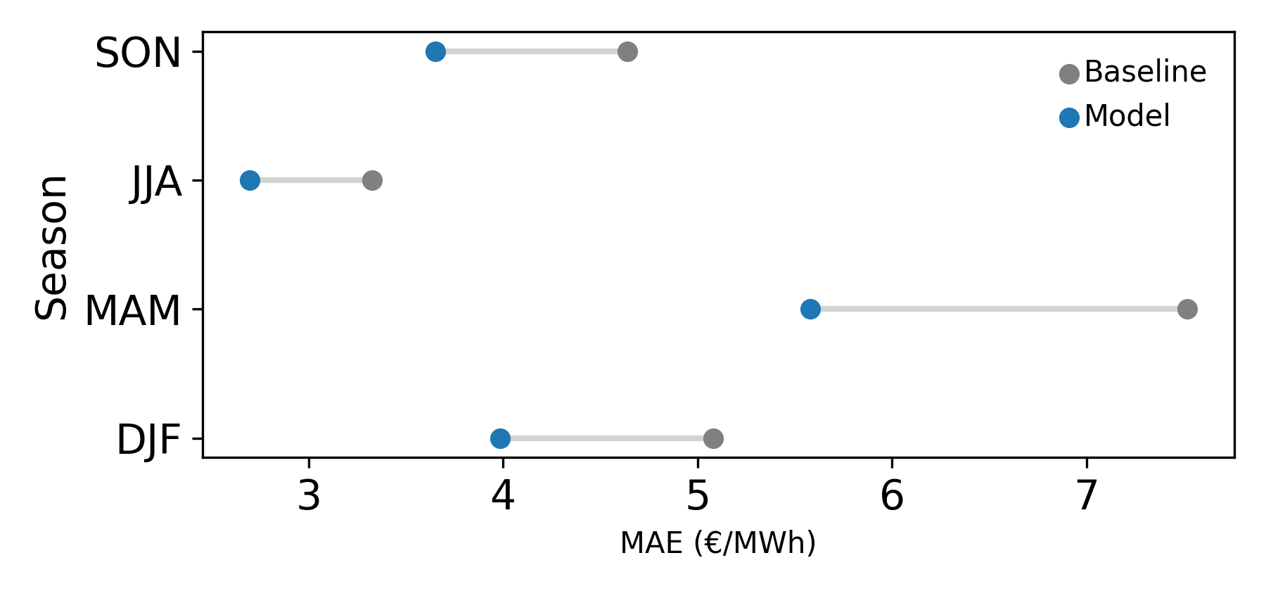
Figure 7 shows seasonal performance, both the baseline and model are strong in the summer months, likely due to the abundance of stable solar power. The spring months sees both model and baseline perform relatively poorly, where weather is likely changeable and wind may dominate more than in summer.
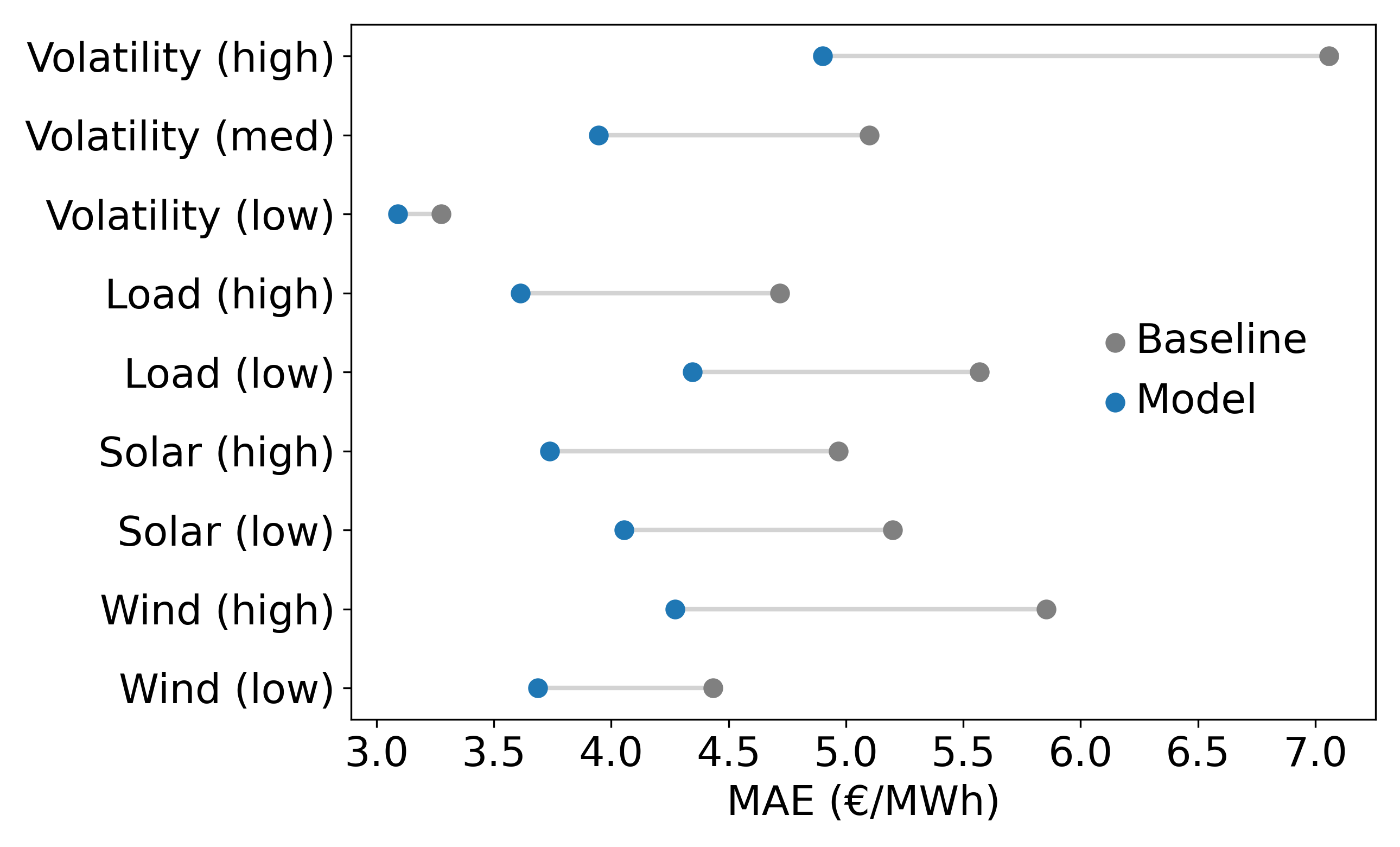
Figure 8 shows a number of regimes. We can see the model and baseline perform worse in low load scenarios, which likely coincide with higher renewable share of generation. One notable result is that the absolute improvement of the model over baseline increases substantially in high wind compared to low wind. We can also see that the baseline struggles on highly volatile days compared to the model, indicating the model is able to derive pricing signals from generation quite well.
Figure 9 shows model predictions vs actual on the test data. If we assume a similar distribution on the training data, more data is available at higher prices which is why the model performs better in that range. As the price decreases we can see from the scatter data that the plot becomes more sparse, and the error increases accordingly.
Protocol
Unless otherwise stated, this is the setup used for all development, testing and evaluation.
Training and evaluation runs were performed using Modal[6]. To keep the resources in-line with Google Colab free tier, runs were configured with a maximum of 2vCPUs, 12GB RAM and 1xT4 GPU. A timeout of 8 hours was configured to ensure all runs were within computational limits imposed. Any metrics shown or discussed were collected and stored using wandb[7].
Any experiments on multiple seeds were gathered over 3 seeds, unless otherwise noted. All runs had 300 maximum epochs, with an early termination if validation scores did not improve in the last 30 epochs. The weights generated by the best run are classed as the output model for that run.
Hyperparameter Optimisation
Initial values for the model were hand-tuned during development whilst the final model was still being decided. When the model shape produced satisfactory results, a round of optimisation was performed to tune the parameters, using the values found manually as a starting point.
To remain within compute limits the optimisation was performed in three stages. Firstly structural, to decide on layer sizes and regularisation levels. A small run of 60 experiments was performed using Optuna[8] to intelligently search for the most optimal settings. Secondly, a run of 60 experiments was performed to determine optimiser settings (learning rate & weight decay). Thirdly we performed a grid search of values to determine how much data was provided as input, i.e. number of hours historical data and the stride used when generating historical sequences.
The search to improve optimiser settings did not yield any concrete gains, so are omitted from the following table:
| Name | Best avg val loss |
|---|---|
| Base model | 0.1649 ± 0.0082 |
| Structural | 0.1593 ± 0.0045 |
| Data | 0.1462 ± 0.0025 |
The data optimisation brought notable gains. We can see from the following heatmap that there is a general shape to the performance of each value combination. These are single-seed runs so only give us an indication of performance.
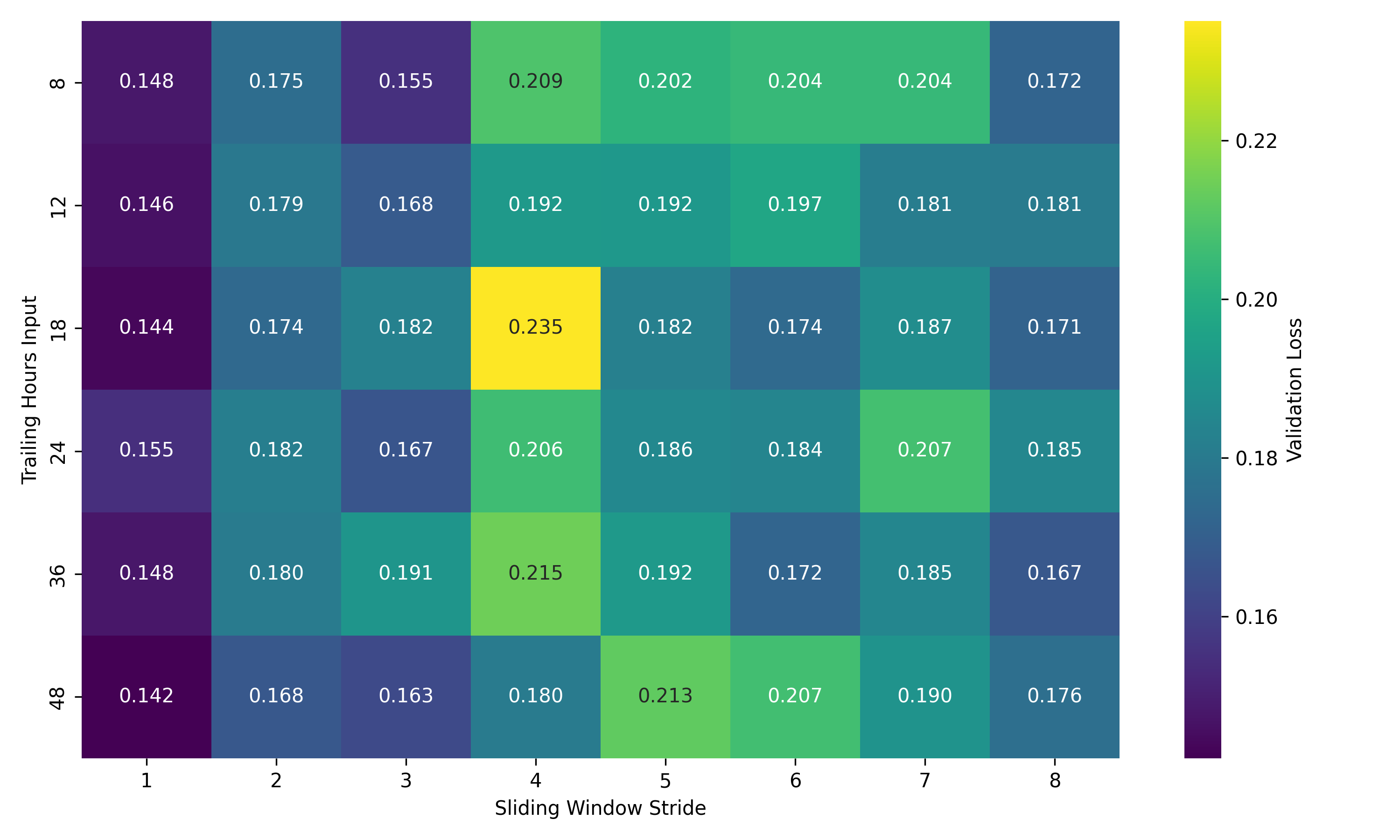
Smaller window strides tend to perform better which is unsurprising, as this leads to the most amount of data being available for training and prevents gaps between sequences. We can also see some underperforming clusters of combinations, e.g. only providing 8 hours of historical data and a large stride. To decide on values for these variables, a further run was performed with a stride of 1, and 3 seeds for each trailing hours input value. The results showed both 18 and 48 performing best, with 18 having lower standard deviation.
Ablations
The following ablations were performed to give an indication of the performance of each component of the model. For CNN and LSTM alterations, layer sizes were increased to control for model capacity. For CNN only ablations the LSTM was replaced with a linear layer to allow shape manip- ulation consistent with the rest of the base model.
| Name | Best Avg Val Loss (MSE) | Parameters |
|---|---|---|
| Base model | 0.1462 ± 0.0025 | 1,264,992 |
| No future weather | 0.1863 ± 0.0021 | 773,976 |
| Pooled future weather | 0.1484 ± 0.0040 | 1,264,728 |
| No historical prices | 0.3518 ± 0.0200 | 1,260,252 |
| No fossil generation | 0.1457 ± 0.0039 | 1,258,720 |
| CNN only | 0.1558 ± 0.0017 | 1,233,056 |
| LSTM only | 0.1654 ± 0.0016 | 1,041,888 |
The weather ablations show the model is able to use future weather predictions effectively, with a 27% increase in MSE when future weather prediction is removed entirely. Pooling only causes a small increase in MSE (approximately 1.5%) and the standard deviations overlap substantially implying there is little performance impact.
For historical prices, we ensured a fair test by passing the prices through the model via the historical CNN+LSTM branch instead of directly into the concatenation layer. The results show a huge increase (approximately 140%) in MSE, suggesting that the model struggled to pick up the price signal compared to the other features. This component is critical to model performance.
A test was performed that removes non-renewables from the historical generation data entirely. The results show a modest improvement over the base model, but with substantial overlap across seeds. The result suggests that renewables capture a larger share of short-term variability compared to fossil fuels. The requirements specify we should avoid excessive feature engineering, so we include this for testing purposes only, the evaluation model uses all generation features and we rely on the model itself to determine which generation features are valuable. We can conclude from the close nature of the results that it does this effectively.
The CNN only results show an approximate 6.6% MSE increase, suggesting the model uses the LSTM to some degree to model longer term trends. Correspondingly the removal of the CNN shows an approximate 13% increase in MSE suggesting the CNN’s role performing local pattern detection is an important one. The combination of both delivers a considerable reduction in MSE as seen in the base model.
Efficiency
These experiments were performed across all available data, and did not inform model choice for training or evaluation.
The base model was trained with mixed precision to determine effects on training and inference performance.
| Name | Val Loss (MSE) | Eval MAE | Eval MSE | Eval MAPE |
|---|---|---|---|---|
| Base | 0.1462 ± 0.0025 | 3.9795 | 5.4034 | 7.31 |
| Mixed | 0.1456 ± 0.0026 | 4.0726 | 5.4914 | 7.42 |
The mixed precision model performs well on training, with comparable results to the base model. There is a slight reduction in performance on the eval data however, suggesting the resulting model did not generalise quite as well, likely due to the reduced numerical precision or the accumulation of rounding errors.
When we consider the efficiency differences in training however:
| Name | Training (sec/it) | Max allocated GPU mem (%) |
|---|---|---|
| Base | 6.9096 ± 0.0537 | 36.2470 ± 0.0075 |
| Mixed | 2.9857 ± 0.0122 | 16.82861 ± 0 |
Mixed precision substantially improves training efficiency, reducing per-iteration latency by more than half with very small variance across seeds. The GPU memory utilisation is only what is allocated rather than what was used so acts as an upper bound, but we can see the mixed precision model required less than half the memory of the base model.
If we consider the large training gains against the relatively minor inference performance loss, it’s conceivable that in a real-world setting we might choose mixed precision as the default model.
We briefly explored inference-time quantisation, but as it did not yield improvements, it was not pursued further. Inference time for the evaluation model was measured on CPU during result gener- ation, with a single forward pass producing the full 24-hour forecast taking approximately 1–2 ms. Given the once-daily forecasting cadence, inference latency does not represent a practical bottleneck in this setting.
Conclusion
The model shows a clear improvement over all baselines, especially in times of high volatility. Ablation studies show the model is particularly sensitive to the inclusion of historical prices at a later stage in the architecture, and various methods of handling future weather predictions offer comparatively smaller, though consistent, improvements.
One area for further research would be to alter the architecture to reduce the dominance of historical prices. Preliminary experiments explored models that attempted to predict the difference from the price at the same hour yesterday, rather than a raw price (i.e. time series differencing) but the models were reluctant to deviate too much from that value. It’s possible the injection of prices so late in the model is having a similar (albeit less pronounced) effect.
Given fewer compute constraints, more exploration of hyperparameter settings would be valuable. Whilst the staged optimisation strategy used here enabled effective tuning within the resource limits, a joint optimisation over architectural, optimisation and data-related parameters may uncover additional high-performing configurations that were missed in our staged approach, due to focusing on local minima in the preceding stage.
In summary, this work shows that a deep learning model can effectively learn the relationship between weather-driven generation, demand patterns and electricity prices under the assumption of perfect future weather forecasts, with particularly strong performance in volatile regimes.